python使用梯度下降算法实现一个多线性回归,供大家参考,具体内容如下
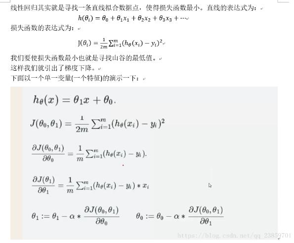
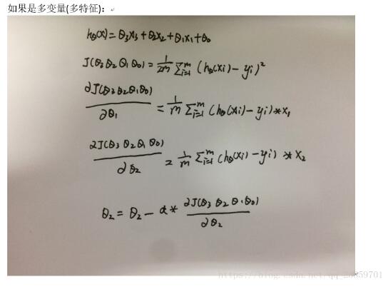
图示:


import pandas as pd
import matplotlib.pylab as plt
import numpy as np
# Read data from csv
pga = pd.read_csv("D:\python3\data\Test.csv")
# Normalize the data 归一化值 (x - mean) / (std)
pga.AT = (pga.AT - pga.AT.mean()) / pga.AT.std()
pga.V = (pga.V - pga.V.mean()) / pga.V.std()
pga.AP = (pga.AP - pga.AP.mean()) / pga.AP.std()
pga.RH = (pga.RH - pga.RH.mean()) / pga.RH.std()
pga.PE = (pga.PE - pga.PE.mean()) / pga.PE.std()


def cost(theta0, theta1, theta2, theta3, theta4, x1, x2, x3, x4, y):
 # Initialize cost
 J = 0
 # The number of observations
 m = len(x1)
 # Loop through each observation
 # 通过每次观察进行循环
 for i in range(m):
 # Compute the hypothesis
 # 计算假设
 h=theta0+x1[i]*theta1+x2[i]*theta2+x3[i]*theta3+x4[i]*theta4
 # Add to cost
 J += (h - y[i])**2
 # Average and normalize cost
 J /= (2*m)
 return J
# The cost for theta0=0 and theta1=1


def partial_cost_theta4(theta0,theta1,theta2,theta3,theta4,x1,x2,x3,x4,y):
 h = theta0 + x1 * theta1 + x2 * theta2 + x3 * theta3 + x4 * theta4
 diff = (h - y) * x4
 partial = diff.sum() / (x2.shape[0])
 return partial


def partial_cost_theta3(theta0,theta1,theta2,theta3,theta4,x1,x2,x3,x4,y):
 h = theta0 + x1 * theta1 + x2 * theta2 + x3 * theta3 + x4 * theta4
 diff = (h - y) * x3
 partial = diff.sum() / (x2.shape[0])
 return partial


def partial_cost_theta2(theta0,theta1,theta2,theta3,theta4,x1,x2,x3,x4,y):
 h = theta0 + x1 * theta1 + x2 * theta2 + x3 * theta3 + x4 * theta4
 diff = (h - y) * x2
 partial = diff.sum() / (x2.shape[0])
 return partial


def partial_cost_theta1(theta0,theta1,theta2,theta3,theta4,x1,x2,x3,x4,y):
 h = theta0 + x1 * theta1 + x2 * theta2 + x3 * theta3 + x4 * theta4
 diff = (h - y) * x1
 partial = diff.sum() / (x2.shape[0])
 return partial

# 对theta0 进行求导
# Partial derivative of cost in terms of theta0


def partial_cost_theta0(theta0, theta1, theta2, theta3, theta4, x1, x2, x3, x4, y):
 h = theta0 + x1 * theta1 + x2 * theta2 + x3 * theta3 + x4 * theta4
 diff = (h - y)
 partial = diff.sum() / (x2.shape[0])
 return partial


def gradient_descent(x1,x2,x3,x4,y, alpha=0.1, theta0=0, theta1=0,theta2=0,theta3=0,theta4=0):
 max_epochs = 1000 # Maximum number of iterations 最大迭代次数
 counter = 0 # Intialize a counter 当前第几次
 c = cost(theta0, theta1, theta2, theta3, theta4, x1, x2, x3, x4, y) ## Initial cost 当前代价函数
 costs = [c] # Lets store each update 每次损失值都记录下来
 # Set a convergence threshold to find where the cost function in minimized
 # When the difference between the previous cost and current cost
 # is less than this value we will say the parameters converged
 # 设置一个收敛的阈值 (两次迭代目标函数值相差没有相差多少,就可以停止了)
 convergence_thres = 0.000001
 cprev = c + 10
 theta0s = [theta0]
 theta1s = [theta1]
 theta2s = [theta2]
 theta3s = [theta3]
 theta4s = [theta4]
 # When the costs converge or we hit a large number of iterations will we stop updating
 # 两次间隔迭代目标函数值相差没有相差多少(说明可以停止了)
 while (np.abs(cprev - c) > convergence_thres) and (counter < max_epochs):
 cprev = c
 # Alpha times the partial deriviative is our updated
 # 先求导, 导数相当于步长
 update0 = alpha * partial_cost_theta0(theta0, theta1, theta2, theta3, theta4, x1, x2, x3, x4, y)
 update1 = alpha * partial_cost_theta1(theta0, theta1, theta2, theta3, theta4, x1, x2, x3, x4, y)
 update2 = alpha * partial_cost_theta2(theta0, theta1, theta2, theta3, theta4, x1, x2, x3, x4, y)
 update3 = alpha * partial_cost_theta3(theta0, theta1, theta2, theta3, theta4, x1, x2, x3, x4, y)
 update4 = alpha * partial_cost_theta4(theta0, theta1, theta2, theta3, theta4, x1, x2, x3, x4, y)
 # Update theta0 and theta1 at the same time
 # We want to compute the slopes at the same set of hypothesised parameters
 #  so we update after finding the partial derivatives
 # -= 梯度下降,+=梯度上升
 theta0 -= update0
 theta1 -= update1
 theta2 -= update2
 theta3 -= update3
 theta4 -= update4

 # Store thetas
 theta0s.append(theta0)
 theta1s.append(theta1)
 theta2s.append(theta2)
 theta3s.append(theta3)
 theta4s.append(theta4)

 # Compute the new cost
 # 当前迭代之后,参数发生更新
 c = cost(theta0, theta1, theta2, theta3, theta4, x1, x2, x3, x4, y)

 # Store updates,可以进行保存当前代价值
 costs.append(c)
 counter += 1 # Count
 # 将当前的theta0, theta1, costs值都返回去
 #return {'theta0': theta0, 'theta1': theta1, 'theta2': theta2, 'theta3': theta3, 'theta4': theta4, "costs": costs}
 return {'costs':costs}

print("costs =", gradient_descent(pga.AT, pga.V,pga.AP,pga.RH,pga.PE)['costs'])
descend = gradient_descent(pga.AT, pga.V,pga.AP,pga.RH,pga.PE, alpha=.01)
plt.scatter(range(len(descend["costs"])), descend["costs"])
plt.show()
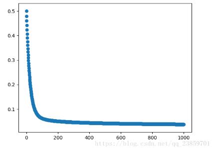
损失函数随迭代次数变换图:

以上就是本文的全部内容,希望对大家的学习有所帮助,也希望大家多多支持自学编程网。

- 本文固定链接: https://zxbcw.cn/post/183418/
- 转载请注明:必须在正文中标注并保留原文链接
- QQ群: PHP高手阵营官方总群(344148542)
- QQ群: Yii2.0开发(304864863)
