
本文实例为大家分享了pytorch实现逻辑回归的具体代码,供大家参考,具体内容如下
一、pytorch实现逻辑回归
逻辑回归是非常经典的分类算法,是用于分类任务,如垃圾分类任务,情感分类任务等都可以使用逻辑回归。
接下来使用逻辑回归模型完成一个二分类任务:
# 使用逻辑回归完成一个二分类任务
# 数据准备
import torch
import matplotlib.pyplot as plt
x1 = torch.randn(365)+1.5 # randn():输出一个形状为size的标准正态分布Tensor
x2 = torch.randn(365)-1.5
#print(x1.shape) # torch.Size([365])
#print(x2.shape) # torch.Size([365])
data = zip(x1.data.numpy(),x2.data.numpy()) # 创建一个聚合了来自每个可迭代对象中的元素的迭代器。 x = [1,2,3]
pos = []
neg = []
def classification(data):
for i in data:
if (i[0] > 1.5+0.1*torch.rand(1).item()*(-1)**torch.randint(1,10,(1,1)).item()):
pos.append(i)
else:
neg.append(i)
classification(data)
# 将正、负两类数据可视化
pos_x = [i[0] for i in pos]
pos_y = [i[1] for i in pos]
neg_x = [i[0] for i in neg]
neg_y = [i[1] for i in neg]
plt.scatter(pos_x,pos_y,c = 'r',marker = "*")
plt.scatter(neg_x,neg_y,c = 'b',marker = "^")
plt.show()
# 构造正、负两类数据可视化结果如上图所示
# 构建模型
import torch.nn as nn
class LogisticRegression(nn.Module):
def __init__(self):
super(LogisticRegression, self).__init__()
self.linear = nn.Linear(2,1)
self.sigmoid = nn.Sigmoid()
def forward(self,x):
return self.sigmoid(self.linear(x))
model = LogisticRegression()
criterion = nn.BCELoss()
optimizer = torch.optim.SGD(model.parameters(),0.01)
epoch = 5000
features = [[i[0],i[1]] for i in pos]
features.extend([[i[0],i[1]] for i in neg]) #extend 接受一个参数,这个参数总是一个 list,并且把这个 list 中的每个元素添加到原 list 中
features = torch.Tensor(features) # torch.Tensor 生成单精度浮点类型的张量
label = [1 for i in range(len(pos))]
label.extend(0 for i in range(len(neg)))
label = torch.Tensor(label)
print(label.shape)
for i in range(500000):
out = model(features)
#print(out.shape)
loss = criterion(out.squeeze(1),label)
optimizer.zero_grad()
loss.backward()
optimizer.step()
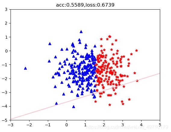
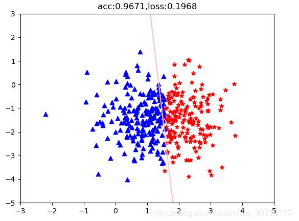
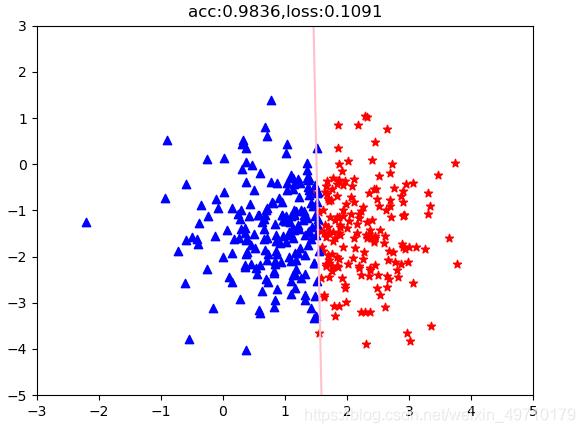
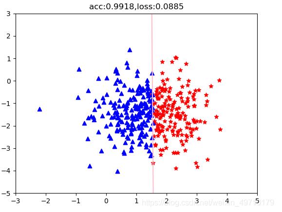
# 分类任务准确率
acc = (out.ge(0.5).float().squeeze(1)==label).sum().float()/features.size()[0]
if (i % 10000 ==0):
plt.scatter(pos_x, pos_y, c='r', marker="*")
plt.scatter(neg_x, neg_y, c='b', marker="^")
weight = model.linear.weight[0]
#print(weight.shape)
wo = weight[0]
w1 = weight[1]
b = model.linear.bias.data[0]
# 绘制分界线
test_x = torch.linspace(-10,10,500) # 500个点
test_y = (-wo*test_x - b) / w1
plt.plot(test_x.data.numpy(),test_y.data.numpy(),c="pink")
plt.title("acc:{:.4f},loss:{:.4f}".format(acc,loss))
plt.ylim(-5,3)
plt.xlim(-3,5)
plt.show()
附上分类结果:
以上就是本文的全部内容,希望对大家的学习有所帮助,也希望大家多多支持自学编程网。

- 本文固定链接: https://zxbcw.cn/post/209236/
- 转载请注明:必须在正文中标注并保留原文链接
- QQ群: PHP高手阵营官方总群(344148542)
- QQ群: Yii2.0开发(304864863)