
1 Support Vector Machines
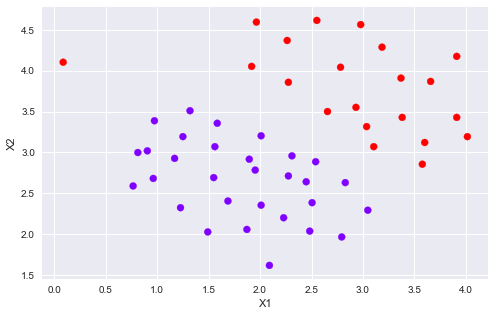
1.1 Example Dataset 1
%matplotlib inline
import numpy as np
import pandas as pd
import matplotlib.pyplot as plt
import seaborn as sb
from scipy.io import loadmat
from sklearn import svm
大多数SVM的库会自动帮你添加额外的特征X₀已经θ₀,所以无需手动添加
mat = loadmat('./data/ex6data1.mat')
print(mat.keys())
# dict_keys(['__header__', '__version__', '__globals__', 'X', 'y'])
X = mat['X']
y = mat['y']
def plotData(X, y):
    plt.figure(figsize=(8,5))
    plt.scatter(X[:,0], X[:,1], c=y.flatten(), cmap='rainbow')
    plt.xlabel('X1')
    plt.ylabel('X2')
    plt.legend()
plotData(X, y)
def plotBoundary(clf, X):
    '''plot decision bondary'''
    x_min, x_max = X[:,0].min()*1.2, X[:,0].max()*1.1
    y_min, y_max = X[:,1].min()*1.1,X[:,1].max()*1.1
    xx, yy = np.meshgrid(np.linspace(x_min, x_max, 500),
                         np.linspace(y_min, y_max, 500))
    Z = clf.predict(np.c_[xx.ravel(), yy.ravel()])
    Z = Z.reshape(xx.shape)
    plt.contour(xx, yy, Z)
models = [svm.SVC(C, kernel='linear') for C in [1, 100]]
clfs = [model.fit(X, y.ravel()) for model in models]
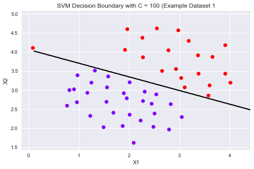
title = ['SVM Decision Boundary with C = {} (Example Dataset 1'.format(C) for C in [1, 100]]
for model,title in zip(clfs,title):
    plt.figure(figsize=(8,5))
    plotData(X, y)
    plotBoundary(model, X)
    plt.title(title)
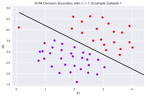
可以从上图看到,当C比较小时模型对误分类的惩罚增大,比较严格,误分类少,间隔比较狭窄。
当C比较大时模型对误分类的惩罚增大,比较宽松,允许一定的误分类存在,间隔较大。
1.2 SVM with Gaussian Kernels
这部分,使用SVM做非线性分类。我们将使用高斯核函数。
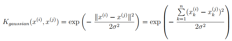
为了用SVM找出一个非线性的决策边界,我们首先要实现高斯核函数。我可以把高斯核函数想象成一个相似度函数,用来测量一对样本的距离,(x ⁽ ʲ ⁾,y ⁽ ⁱ ⁾)
这里我们用sklearn自带的svm中的核函数即可。
1.2.1 Gaussian Kernel
def gaussKernel(x1, x2, sigma):
    return np.exp(- ((x1 - x2) ** 2).sum() / (2 * sigma ** 2))
gaussKernel(np.array([1, 2, 1]),np.array([0, 4, -1]), 2.)  # 0.32465246735834974
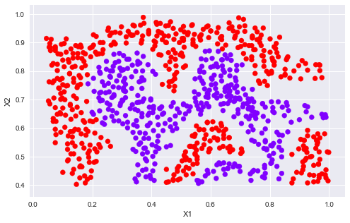
1.2.2 Example Dataset 2
mat = loadmat('./data/ex6data2.mat')
X2 = mat['X']
y2 = mat['y']
plotData(X2, y2)
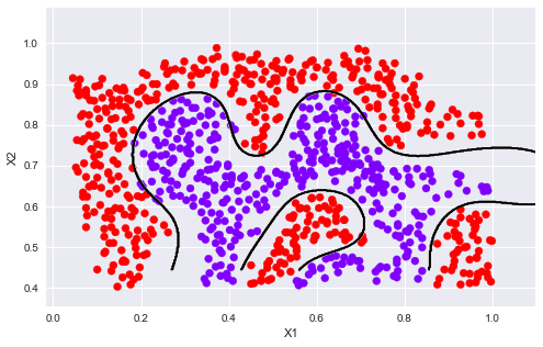
sigma = 0.1
gamma = np.power(sigma,-2.)/2
clf = svm.SVC(C=1, kernel='rbf', gamma=gamma)
modle = clf.fit(X2, y2.flatten())
plotData(X2, y2)
plotBoundary(modle, X2)
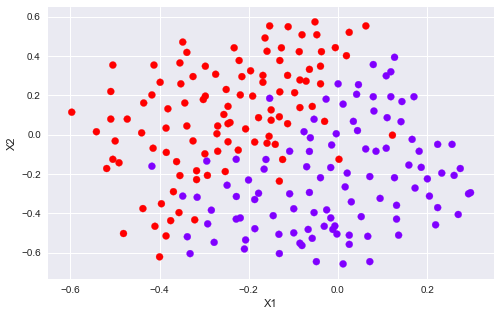
1.2.3 Example Dataset 3
mat3 = loadmat('data/ex6data3.mat')
X3, y3 = mat3['X'], mat3['y']
Xval, yval = mat3['Xval'], mat3['yval']
plotData(X3, y3)
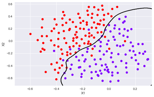
Cvalues = (0.01, 0.03, 0.1, 0.3, 1., 3., 10., 30.)
sigmavalues = Cvalues
best_pair, best_score = (0, 0), 0
for C in Cvalues:
    for sigma in sigmavalues:
        gamma = np.power(sigma,-2.)/2
        model = svm.SVC(C=C,kernel='rbf',gamma=gamma)
        model.fit(X3, y3.flatten())
        this_score = model.score(Xval, yval)
        if this_score > best_score:
            best_score = this_score
            best_pair = (C, sigma)
print('best_pair={}, best_score={}'.format(best_pair, best_score))
# best_pair=(1.0, 0.1), best_score=0.965
model = svm.SVC(C=1., kernel='rbf', gamma = np.power(.1, -2.)/2)
model.fit(X3, y3.flatten())
plotData(X3, y3)
plotBoundary(model, X3)
# 这我的一个练习画图的,和作业无关,给个画图的参考。
import numpy as np
import matplotlib.pyplot as plt
from sklearn import svm
# we create 40 separable points
np.random.seed(0)
X = np.array([[3,3],[4,3],[1,1]])
Y = np.array([1,1,-1])
# fit the model
clf = svm.SVC(kernel='linear')
clf.fit(X, Y)
# get the separating hyperplane
w = clf.coef_[0]
a = -w[0] / w[1]
xx = np.linspace(-5, 5)
yy = a * xx - (clf.intercept_[0]) / w[1]
# plot the parallels to the separating hyperplane that pass through the
# support vectors
b = clf.support_vectors_[0]
yy_down = a * xx + (b[1] - a * b[0])
b = clf.support_vectors_[-1]
yy_up = a * xx + (b[1] - a * b[0])
# plot the line, the points, and the nearest vectors to the plane
plt.figure(figsize=(8,5))
plt.plot(xx, yy, 'k-')
plt.plot(xx, yy_down, 'k--')
plt.plot(xx, yy_up, 'k--')
# 圈出支持向量
plt.scatter(clf.support_vectors_[:, 0], clf.support_vectors_[:, 1],
            s=150, facecolors='none', edgecolors='k', linewidths=1.5)
plt.scatter(X[:, 0], X[:, 1], c=Y, cmap=plt.cm.rainbow)
plt.axis('tight')
plt.show()
print(clf.decision_function(X))
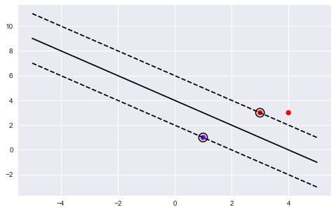
[ 1. 1.5 -1. ]
2 Spam Classification
2.1 Preprocessing Emails
这部分用SVM建立一个垃圾邮件分类器。你需要将每个email变成一个n维的特征向量,这个分类器将判断给定一个邮件x是垃圾邮件(y=1)或不是垃圾邮件(y=0)。
take a look at examples from the dataset
with open('data/emailSample1.txt', 'r') as f:
    email = f.read()
    print(email)
> Anyone knows how much it costs to host a web portal ?
>
Well, it depends on how many visitors you're expecting.
This can be anywhere from less than 10 bucks a month to a couple of $100.
You should checkout http://www.rackspace.com/ or perhaps Amazon EC2
if youre running something big..
To unsubscribe yourself from this mailing list, send an email to:
groupname-unsubscribe@egroups.com
可以看到,邮件内容包含 a URL, an email address(at the end), numbers, and dollar amounts. 很多邮件都会包含这些元素,但是每封邮件的具体内容可能会不一样。因此,处理邮件经常采用的方法是标准化这些数据,把所有URL当作一样,所有数字看作一样。
例如,我们用唯一的一个字符串‘httpaddr'来替换所有的URL,来表示邮件包含URL,而不要求具体的URL内容。这通常会提高垃圾邮件分类器的性能,因为垃圾邮件发送者通常会随机化URL,因此在新的垃圾邮件中再次看到任何特定URL的几率非常小。
我们可以做如下处理:
  1. Lower-casing: 把整封邮件转化为小写。
  2. Stripping HTML: 移除所有HTML标签,只保留内容。
  3. Normalizing URLs: 将所有的URL替换为字符串 “httpaddr”.
  4. Normalizing Email Addresses: 所有的地址替换为 “emailaddr”
  5. Normalizing Dollars: 所有dollar符号($)替换为“dollar”.
  6. Normalizing Numbers: 所有数字替换为“number”
  7. Word Stemming(词干提取): 将所有单词还原为词源。例如,“discount”, “discounts”, “discounted” and “discounting”都替换为“discount”。
  8. Removal of non-words: 移除所有非文字类型,所有的空格(tabs, newlines, spaces)调整为一个空格.
%matplotlib inline
import numpy as np
import matplotlib.pyplot as plt
from scipy.io import loadmat
from sklearn import svm
import re #regular expression for e-mail processing
# 这是一个可用的英文分词算法(Porter stemmer)
from stemming.porter2 import stem
# 这个英文算法似乎更符合作业里面所用的代码,与上面效果差不多
import nltk, nltk.stem.porter
def processEmail(email):
    """做除了Word Stemming和Removal of non-words的所有处理"""
    email = email.lower()
    email = re.sub('<[^<>]>', ' ', email)  # 匹配<开头,然后所有不是< ,> 的内容,知道>结尾,相当于匹配<...>
    email = re.sub('(http|https)://[^\s]*', 'httpaddr', email )  # 匹配//后面不是空白字符的内容,遇到空白字符则停止
    email = re.sub('[^\s]+@[^\s]+', 'emailaddr', email)
    email = re.sub('[\$]+', 'dollar', email)
    email = re.sub('[\d]+', 'number', email)
    return email
接下来就是提取词干,以及去除非字符内容。
def email2TokenList(email):
    """预处理数据,返回一个干净的单词列表"""
    # I'll use the NLTK stemmer because it more accurately duplicates the
    # performance of the OCTAVE implementation in the assignment
    stemmer = nltk.stem.porter.PorterStemmer()
    email = preProcess(email)
    # 将邮件分割为单个单词,re.split() 可以设置多种分隔符
    tokens = re.split('[ \@\$\/\#\.\-\:\&\*\+\=\[\]\?\!\(\)\{\}\,\'\"\>\_\<\;\%]', email)
    # 遍历每个分割出来的内容
    tokenlist = []
    for token in tokens:
        # 删除任何非字母数字的字符
        token = re.sub('[^a-zA-Z0-9]', '', token);
        # Use the Porter stemmer to 提取词根
        stemmed = stemmer.stem(token)
        # 去除空字符串‘',里面不含任何字符
        if not len(token): continue
        tokenlist.append(stemmed)
    return tokenlist
2.1.1 Vocabulary List(词汇表)
在对邮件进行预处理之后,我们有一个处理后的单词列表。下一步是选择我们想在分类器中使用哪些词,我们需要去除哪些词。
我们有一个词汇表vocab.txt,里面存储了在实际中经常使用的单词,共1899个。
我们要算出处理后的email中含有多少vocab.txt中的单词,并返回在vocab.txt中的index,这就我们想要的训练单词的索引。
def email2VocabIndices(email, vocab):
    """提取存在单词的索引"""
    token = email2TokenList(email)
    index = [i for i in range(len(vocab)) if vocab[i] in token ]
    return index
2.2 Extracting Features from Emails
def email2FeatureVector(email):
    """
    将email转化为词向量,n是vocab的长度。存在单词的相应位置的值置为1,其余为0
    """
    df = pd.read_table('data/vocab.txt',names=['words'])
    vocab = df.as_matrix()  # return array
    vector = np.zeros(len(vocab))  # init vector
    vocab_indices = email2VocabIndices(email, vocab)  # 返回含有单词的索引
    # 将有单词的索引置为1
    for i in vocab_indices:
        vector[i] = 1
    return vector
vector = email2FeatureVector(email)
print('length of vector = {}\nnum of non-zero = {}'.format(len(vector), int(vector.sum())))
length of vector = 1899
num of non-zero = 45
2.3 Training SVM for Spam Classification
读取已经训提取好的特征向量以及相应的标签。分训练集和测试集。
# Training set
mat1 = loadmat('data/spamTrain.mat')
X, y = mat1['X'], mat1['y']
# Test set
mat2 = scipy.io.loadmat('data/spamTest.mat')
Xtest, ytest = mat2['Xtest'], mat2['ytest']
clf = svm.SVC(C=0.1, kernel='linear')
clf.fit(X, y)
2.4 Top Predictors for Spam
predTrain = clf.score(X, y)
predTest = clf.score(Xtest, ytest)
predTrain, predTest
(0.99825, 0.989)
到此这篇关于机器学习SVM支持向量机的练习文章就介绍到这了,更多相关机器学习内容请搜索自学编程网以前的文章或继续浏览下面的相关文章,希望大家以后多多支持自学编程网!
- 本文固定链接: https://zxbcw.cn/post/209739/
- 转载请注明:必须在正文中标注并保留原文链接
- QQ群: PHP高手阵营官方总群(344148542)
- QQ群: Yii2.0开发(304864863)