OpenCV半小时掌握基本操作之直线检测

概述

OpenCV 是一个跨平台的计算机视觉库, 支持多语言, 功能强大. 今天小白就带大家一起携手走进 OpenCV 的世界. (第 13 课)

在这里插入图片描述

霍夫直线变换

霍夫变换 (Hough Line Transform) 是图像处理中的一种特征提取技术. 通过平面空间到极值坐标空间的转换, 可以帮助我们实现直线检测. 如图:

在这里插入图片描述

原理详解

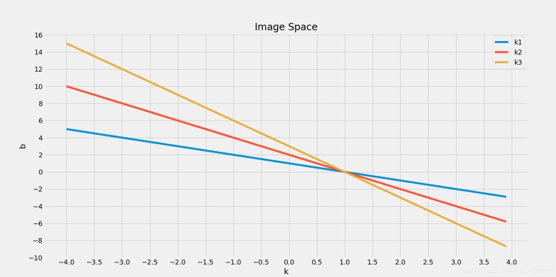
当我们把直线 y = kx + b 画在指标坐标系上, 如下图. 我们再从原点引线段到直线上的任一点.

在这里插入图片描述

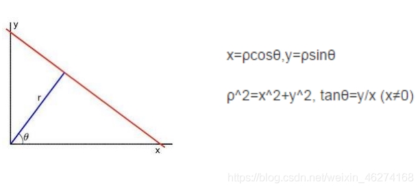
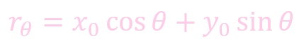
我们可以得到这条线段与 x 轴的夹角为 θ, 距离是 r. 对于直线上的任一点 (x0, y0), 我们可以得到公式:

在这里插入图片描述

代码实战

HoughLines

格式:

cv2.HoughLines(image, rho, theta, threshold, lines=None, srn=None, stn=None, min_theta=None, max_theta=None)

参数:

image: 输入图像
rho: 线性搜索半径步长, 以像素为单位
theta: 线性搜索步长, 以弧度为单位
threshold: 累计阈值

例子:

import numpy as np
import cv2
from matplotlib import pyplot as plt

# 读取图片
image = cv2.imread("sudoku.jpg")
image_copy = image.copy()

# 转换成灰度图
image_gray = cv2.cvtColor(image, cv2.COLOR_BGR2GRAY)

# 边缘检测, Sobel算子大小为3
edges = cv2.Canny(image_gray, 170, 220, apertureSize=3)

# 霍夫曼直线检测
lines = cv2.HoughLines(edges, 1, np.pi / 180, 250)

# 遍历
for line in lines:
    # 获取rho和theta
    rho, theta = line[0]
    a = np.cos(theta)
    b = np.sin(theta)
    x0 = a * rho
    y0 = b * rho
    x1 = int(x0 + 1000 * (-b))
    y1 = int(y0 + 1000 * (a))
    x2 = int(x0 - 1000 * (-b))
    y2 = int(y0 - 1000 * (a))
    cv2.line(image_copy, (x1, y1), (x2, y2), (0, 0, 255), thickness=5)

# 图片展示
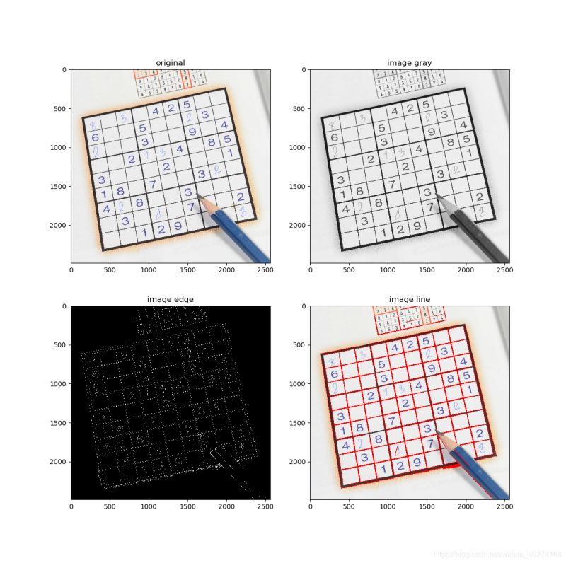
f, ax = plt.subplots(2, 2, figsize=(12, 12))

# 子图
ax[0, 0].imshow(cv2.cvtColor(image, cv2.COLOR_BGR2RGB))
ax[0, 1].imshow(image_gray, "gray")
ax[1, 0].imshow(edges, "gray")
ax[1, 1].imshow(cv2.cvtColor(image_copy, cv2.COLOR_BGR2RGB))

# 标题
ax[0, 0].set_title("original")
ax[0, 1].set_title("image gray")
ax[1, 0].set_title("image edge")
ax[1, 1].set_title("image line")

plt.show()

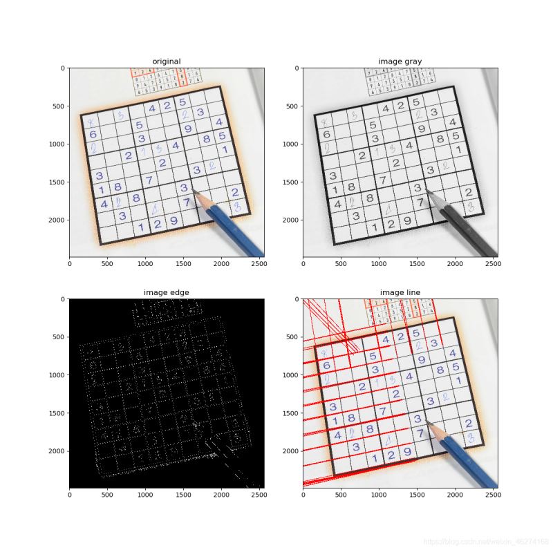
输出结果:

在这里插入图片描述

HoughLinesP

此函数在 HoughLines 的基础上末尾加了一个代表概率 (Probabilistic) 的 P, 表明它可以采用累计概率霍夫变换, 来找出二值图像中的直线.

格式:

HoughLinesP(image, rho, theta, threshold, lines=None, minLineLength=None, maxLineGap=None)

参数:

image: 输入图像
rho: 线性搜索半径步长, 以像素为单位
theta: 线性搜索步长, 以弧度为单位
threshold: 累计阈值
minLineLength: 最短直线长度
maxLineGap: 最大孔隙距离

例子:

import numpy as np
import cv2
from matplotlib import pyplot as plt

# 读取图片
image = cv2.imread("sudoku.jpg")
image_copy = image.copy()

# 转换成灰度图
image_gray = cv2.cvtColor(image, cv2.COLOR_BGR2GRAY)

# 边缘检测, Sobel算子大小为3
edges = cv2.Canny(image_gray, 170, 220, apertureSize=3)

# 霍夫曼直线检测
lines = cv2.HoughLinesP(edges, 1, np.pi / 180, 100, minLineLength=100, maxLineGap=10)

# 遍历
for line in lines:

    # 获取坐标
    x1, y1, x2, y2 = line[0]
    cv2.line(image_copy, (x1, y1), (x2, y2), (0, 0, 255), thickness=5)


# 图片展示
f, ax = plt.subplots(2, 2, figsize=(12, 12))

# 子图
ax[0, 0].imshow(cv2.cvtColor(image, cv2.COLOR_BGR2RGB))
ax[0, 1].imshow(image_gray, "gray")
ax[1, 0].imshow(edges, "gray")
ax[1, 1].imshow(cv2.cvtColor(image_copy, cv2.COLOR_BGR2RGB))

# 标题
ax[0, 0].set_title("original")
ax[0, 1].set_title("image gray")
ax[1, 0].set_title("image edge")
ax[1, 1].set_title("image line")

plt.show()

输出结果:

在这里插入图片描述

到此这篇关于OpenCV半小时掌握基本操作之直线检测的文章就介绍到这了,更多相关OpenCV直线检测内容请搜索自学编程网以前的文章或继续浏览下面的相关文章希望大家以后多多支持自学编程网！

编程技巧

目录

概述

霍夫直线变换

原理详解

代码实战

HoughLines

HoughLinesP